机器学习——支持向量机(SVM)
支持向量机原理
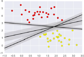
支持向量机要解决的问题其实就是寻求最优分类边界。且最大化支持向量间距,用直线或者平面,分隔分隔超平面。
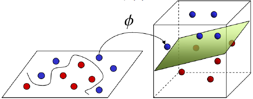
基于核函数的升维变换
通过名为核函数的特征变换,增加新的特征,使得低维度空间中的线性不可分问题变为高维度空间中的线性可分问题。
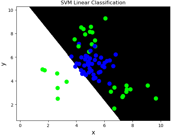
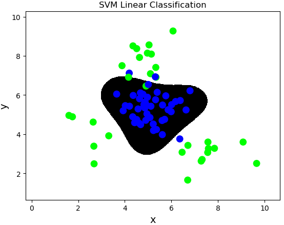
线性核函数:linear,不通过核函数进行维度提升,仅在原始维度空间中寻求线性分类边界。
基于线性核函数的SVM分类相关API:
import sklearn.svm as svm
model = svm.SVC(kernel='linear')
model.fit(train_x, train_y)
案例:对multiple2.txt中的数据进行分类。
import numpy as np
import sklearn.model_selection as ms
import sklearn.svm as svm
import sklearn.metrics as sm
import matplotlib.pyplot as mp
x, y = [], []
data = np.loadtxt('../data/multiple2.txt', delimiter=',', dtype='f8')
x = data[:, :-1]
y = data[:, -1]
train_x, test_x, train_y, test_y = \
    ms.train_test_split(x, y, test_size=0.25, random_state=5)
# 基于线性核函数的支持向量机分类器
model = svm.SVC(kernel='linear')
model.fit(train_x, train_y)
n = 500
l, r = x[:, 0].min() - 1, x[:, 0].max() + 1
b, t = x[:, 1].min() - 1, x[:, 1].max() + 1
grid_x = np.meshgrid(np.linspace(l, r, n),
                     np.linspace(b, t, n))
flat_x = np.column_stack((grid_x[0].ravel(), grid_x[1].ravel()))
flat_y = model.predict(flat_x)
grid_y = flat_y.reshape(grid_x[0].shape)
pred_test_y = model.predict(test_x)
cr = sm.classification_report(test_y, pred_test_y)
print(cr)
mp.figure('SVM Linear Classification', facecolor='lightgray')
mp.title('SVM Linear Classification', fontsize=20)
mp.xlabel('x', fontsize=14)
mp.ylabel('y', fontsize=14)
mp.tick_params(labelsize=10)
mp.pcolormesh(grid_x[0], grid_x[1], grid_y, cmap='gray')
mp.scatter(test_x[:, 0], test_x[:, 1], c=test_y, cmap='brg', s=80)
mp.show()
多项式核函数:poly,通过多项式函数增加原始样本特征的高次方幂
$$y = x_1+x_2 \\
y = x_1^2 + 2x_1x_2 + x_2^2 \\
y = x_1^3 + 3x_1^2x_2 + 3x_1x_2^2 + x_2^3$$
案例,基于多项式核函数训练sample2.txt中的样本数据。
# 基于线性核函数的支持向量机分类器
model = svm.SVC(kernel='poly', degree=3)
model.fit(train_x, train_y)
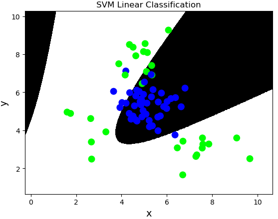
径向基核函数:rbf,通过高斯分布函数增加原始样本特征的分布概率
案例,基于径向基核函数训练sample2.txt中的样本数据。
# 基于径向基核函数的支持向量机分类器
# C:正则强度
# gamma:正态分布曲线的标准差
model = svm.SVC(kernel='rbf', C=600, gamma=0.01)
model.fit(train_x, train_y)
样本类别均衡化
样本类别均衡化:通过类别权重的均衡化,使所占比例较小的样本权重较高,而所占比例较大的样本权重较低,以此平均化不同类别样本对分类模型的贡献,提高模型性能。
样本类别均衡化相关API:
model = svm.SVC(kernel='linear', class_weight='balanced')
model.fit(train_x, train_y)
案例:修改线性核函数的支持向量机案例,基于样本类别均衡化读取imbalance.txt训练模型。
import numpy as np
import sklearn.model_selection as ms
import sklearn.svm as svm
import sklearn.metrics as sm
import matplotlib.pyplot as mp

data = np.loadtxt('../machine_learning_date/imbalance.txt', delimiter=',', dtype='f8')
x = data[:, :-1]
y = data[:, -1]
# 选择svm做分类
train_x, test_x, train_y, test_y = ms.train_test_split(x, y, test_size=0.25, random_state=5)
model = svm.SVC(kernel='linear', class_weight='balanced')
# model = svm.SVC(kernel='linear', class_weight={0:10,1:1})     # 0类别权重为10,1类别权重为1.
model.fit(train_x, train_y)
pred_test_y = model.predict(test_x)
print(sm.classification_report(test_y, pred_test_y))

# 绘制分类边界线
n = 500
l, r = x[:, 0].min() - 1, x[:, 0].max() + 1
b, t = x[:, 1].min() - 1, x[:, 1].max() + 1
grid_x = np.meshgrid(np.linspace(l, r, n), np.linspace(b, t, n))
flat_x = np.column_stack((grid_x[0].ravel(), grid_x[1].ravel()))
flat_y = model.predict(flat_x)
grid_y = flat_y.reshape(grid_x[0].shape)

mp.figure('Class Balanced', facecolor='lightgray')
mp.title('Class Balanced', fontsize=20)
mp.xlabel('x', fontsize=14)
mp.ylabel('y', fontsize=14)
mp.tick_params(labelsize=10)
mp.pcolormesh(grid_x[0], grid_x[1], grid_y, cmap='gray')
mp.scatter(x[:, 0], x[:, 1], c=y, cmap='brg', s=80)
mp.show()

#              precision    recall  f1-score   support
#
#         0.0       0.29      0.76      0.42        42
#         1.0       0.95      0.70      0.80       258
#
# avg / total       0.86      0.71      0.75       300

置信概率
置信概率:根据样本与分类边界的距离远近,对其预测类别的可信程度进行量化,离边界越近的样本,置信概率越低,反之,离边界越远的样本,置信概率高。
获取每个样本的置信概率相关API:
# 在获取模型时,给出超参数probability=True
model = svm.SVC(kernel='rbf', C=600, gamma=0.01, probability=True)
预测结果 = model.predict(输入样本矩阵)
# 调用model.predict_proba(样本矩阵)可以获取每个样本的置信概率矩阵
置信概率矩阵 = model.predict_proba(输入样本矩阵)
置信概率矩阵格式如下:
| 类别1 | 类别2 | |
|---|---|---|
| 样本1 | 0.8 | 0.2 |
| 样本2 | 0.9 | 0.1 |
| 样本3 | 0.5 | 0.5 |
案例:修改基于径向基核函数的SVM案例,新增测试样本,输出每个测试样本的执行概率,并给出标注。
# 新增样本
prob_x = np.array([[2, 1.5], [8, 9], [4.8, 5.2], [4, 4], [2.5, 7], [7.6, 2], [5.4, 5.9]])
pred_prob_y = model.predict(prob_x)
probs = model.predict_proba(prob_x)
print(probs)
# [[3.00000090e-14 1.00000000e+00]
#  [3.00000090e-14 1.00000000e+00]
#  [9.73038186e-01 2.69618143e-02]
#  [5.65786038e-01 4.34213962e-01]
#  [2.77725531e-03 9.97222745e-01]
#  [2.91704904e-11 1.00000000e+00]
#  [9.43796673e-01 5.62033274e-02]]

# 绘制分类边界线
n = 500
l, r = x[:, 0].min() - 1, x[:, 0].max() + 1
b, t = x[:, 1].min() - 1, x[:, 1].max() + 1
grid_x = np.meshgrid(np.linspace(l, r, n), np.linspace(b, t, n))
flat_x = np.column_stack((grid_x[0].ravel(), grid_x[1].ravel()))
flat_y = model.predict(flat_x)
grid_y = flat_y.reshape(grid_x[0].shape)

mp.figure('Probability', facecolor='lightgray')
mp.title('Probability', fontsize=20)
mp.xlabel('x', fontsize=14)
mp.ylabel('y', fontsize=14)
mp.tick_params(labelsize=10)
mp.pcolormesh(grid_x[0], grid_x[1], grid_y, cmap='gray')
mp.scatter(test_x[:, 0], test_x[:, 1], c=test_y, cmap='brg', s=80)
mp.scatter(prob_x[:, 0], prob_x[:, 1], c=pred_prob_y, cmap='jet_r', s=80, marker='D')
# 绘制每个测试样本,并给出标注
for i in range(len(probs)):
    mp.annotate(
        '{}% {}%'.format(
            round(probs[i, 0] * 100, 2),
            round(probs[i, 1] * 100, 2)),
        xy=(prob_x[i, 0], prob_x[i, 1]),
        xytext=(12, -12),
        textcoords='offset points',
        horizontalalignment='left',
        verticalalignment='top',
        fontsize=9,
        bbox={'boxstyle': 'round,pad=0.6', 'fc': 'orange', 'alpha': 0.8})
mp.show()
网格搜索
获取一个最优超参数的方式可以绘制验证曲线,但是验证曲线只能每次获取一个最优超参数。如果多个超参数有很多排列组合的话,就可以使用网格搜索寻求最优超参数组合。
针对超参数组合列表中的每一个超参数组合,实例化给定的模型,做cv次交叉验证,将其中平均f1得分最高的超参数组合作为最佳选择,实例化模型对象。
网格搜索相关API:
import sklearn.model_selection as ms
model = ms.GridSearchCV(模型, 超参数组合列表, cv=折叠数)
model.fit(输入集,输出集)
# 获取网格搜索每个参数组合
model.cv_results_['params']
# 获取网格搜索每个参数组合所对应的平均测试分值
model.cv_results_['mean_test_score']
# 获取最好的参数
model.best_params_   # 最优超参数组合
model.best_score_    # 最优得分
model.best_estimator_  # 最优模型对象
案例:修改置信概率案例,基于网格搜索得到最优超参数。
import numpy as np
import sklearn.model_selection as ms
import sklearn.svm as svm
import sklearn.metrics as sm
import matplotlib.pyplot as plt

data = np.loadtxt('../machine_learning_date/multiple2.txt', delimiter=',', dtype='f8')
x = data[:, :-1]
y = data[:, -1]
# 选择svm做分类
train_x, test_x, train_y, test_y = ms.train_test_split(x, y, test_size=0.25, random_state=5)
model = svm.SVC(probability=True)
# 根据网格搜索选择最优模型
# 整理网格搜索所需要的超参数列表
params = [{'kernel': ['linear'], 'C': [1, 10, 100, 1000]},
          {'kernel': ['poly'], 'C': [1], 'degree': [2, 3]},
          {'kernel': ['rbf'], 'C': [1, 10, 100, 1000], 'gamma': [1, 0.1, 0.01, 0.001]}]
model = ms.GridSearchCV(model, params, cv=5)
model.fit(train_x, train_y)

# 获取得分最优的的超参数信息
print(model.best_params_)  # {'C': 1, 'gamma': 1, 'kernel': 'rbf'}

# 获取最优得分
print(model.best_score_)  # 0.96

# 获取最优模型的信息
print(model.best_estimator_)
# SVC(C=1, cache_size=200, class_weight=None, coef0=0.0,
#   decision_function_shape='ovr', degree=3, gamma=1, kernel='rbf',
#   max_iter=-1, probability=True, random_state=None, shrinking=True,
#   tol=0.001, verbose=False)

# 输出每个超参数组合信息及其得分
for param, score in zip(model.cv_results_['params'], model.cv_results_['mean_test_score']):
    print(param, '->', score)
    # {'C': 1, 'kernel': 'linear'} -> 0.5911111111111111
    # {'C': 10, 'kernel': 'linear'} -> 0.5911111111111111
    # ...
    # ...
    # {'C': 1000, 'gamma': 0.01, 'kernel': 'rbf'} -> 0.9555555555555556
    # {'C': 1000, 'gamma': 0.001, 'kernel': 'rbf'} -> 0.92


pred_test_y = model.predict(test_x)
print(sm.classification_report(test_y, pred_test_y))
#              precision    recall  f1-score   support
#         0.0       0.95      0.93      0.94        45
#         1.0       0.90      0.93      0.92        30
# avg / total       0.93      0.93      0.93        75

# 新增样本
prob_x = np.array([[2, 1.5], [8, 9], [4.8, 5.2], [4, 4], [2.5, 7], [7.6, 2], [5.4, 5.9]])
pred_prob_y = model.predict(prob_x)
probs = model.predict_proba(prob_x)     # 获取每个样本的置信概率矩阵
print(probs)

# 绘制分类边界线
n = 500
l, r = x[:, 0].min() - 1, x[:, 0].max() + 1
b, t = x[:, 1].min() - 1, x[:, 1].max() + 1
grid_x = np.meshgrid(np.linspace(l, r, n), np.linspace(b, t, n))
flat_x = np.column_stack((grid_x[0].ravel(), grid_x[1].ravel()))
flat_y = model.predict(flat_x)
grid_y = flat_y.reshape(grid_x[0].shape)

plt.figure('Probability')
plt.title('Probability')
plt.xlabel('x', fontsize=14)
plt.ylabel('y', fontsize=14)
plt.tick_params(labelsize=10)
plt.pcolormesh(grid_x[0], grid_x[1], grid_y, cmap='gray')
plt.scatter(test_x[:, 0], test_x[:, 1], c=test_y, cmap='brg', s=80)
plt.scatter(prob_x[:, 0], prob_x[:, 1], c=pred_prob_y, cmap='jet_r', s=80, marker='D')
for i in range(len(probs)):
    plt.annotate('{}% {}%'.format(
        round(probs[i, 0] * 100, 2),
        round(probs[i, 1] * 100, 2)),
        xy=(prob_x[i, 0], prob_x[i, 1]),
        xytext=(12, -12),
        textcoords='offset points',
        horizontalalignment='left',
        verticalalignment='top',
        fontsize=9,
        bbox={'boxstyle': 'round,pad=0.6', 'fc': 'orange', 'alpha': 0.8})
plt.show()

事件预测
加载event.txt,预测某个时间段是否会出现特殊事件。
import numpy as np
import sklearn.preprocessing as sp
import sklearn.model_selection as ms
import sklearn.svm as svm
import sklearn.metrics as sm


class DigitEncoder:
    # 模拟LabelEncoder编写的数字编码器
    # 非数字字符串的特征需要做标签编码,
    # 数字字符串的特征需要做转换编码

    def fit_transform(self, y):
        return y.astype('i4')

    def transform(self, y):
        return y.astype('i4')

    def inverse_transform(self, y):
        return y.astype('str')


# 加载并整理数据集
# data = np.load('../machine_learning_date/events.txt', delimiter=",", dtype='U15')

data = []
with open('../machine_learning_date/events.txt', 'r') as f:
    for line in f.readlines():
        data.append(line.split(','))
data = np.array(data)
data = np.delete(data, 1, axis=1)
cols = data.shape[1]  # 获取一共有多少列
x, y = [], []
encoders = []
for i in range(cols):
    col = data[:, i]
    # 判断当前列是否是数字字符串
    if col[0].isdigit():
        encoder = DigitEncoder()
    else:
        encoder = sp.LabelEncoder()
    # 使用编码器对数据进行编码
    if i < cols - 1:
        x.append(encoder.fit_transform(col))
    else:
        y = encoder.fit_transform(col)
    encoders.append(encoder)

x = np.array(x).T   # (5040,4)
y = np.array(y)     # (5040,)

# 拆分测试集与训练集
train_x, test_x, train_y, test_y = ms.train_test_split(x, y, test_size=0.25, random_state=7)

# 构建模型
model = svm.SVC(kernel='rbf', class_weight='balanced')
model.fit(train_x, train_y)
# 测试
pred_test_y = model.predict(test_x)
print(sm.classification_report(test_y, pred_test_y))

# 业务应用
data = [['Tuesday', '13:30:00', '21', '23']]
data = np.array(data).T
x = []
for row in range(len(data)):
    encoder = encoders[row]
    x.append(encoder.transform(data[row]))
x = np.array(x).T
pred_y = model.predict(x)
print(encoders[-1].inverse_transform(pred_y))   # ['eventA\n']
交通流量预测(回归)
加载traffic.txt,预测在某个时间段某个交通路口的车流量。
"""车流量预测"""
import numpy as np
import sklearn.preprocessing as sp
import sklearn.model_selection as ms
import sklearn.svm as svm
import sklearn.metrics as sm


class DigitEncoder:
    def fit_transform(self, y):
        return y.astype(int)

    def transform(self, y):
        return y.astype(int)

    def inverse_transform(self, y):
        return y.astype(str)


data = []
# 回归
data = np.loadtxt('../machine_learning_date/traffic.txt', delimiter=',', dtype='U20')
data = data.T
encoders, x = [], []
for row in range(len(data)):
    if data[row][0].isdigit():
        encoder = DigitEncoder()
    else:
        encoder = sp.LabelEncoder()
    if row < len(data) - 1:
        x.append(encoder.fit_transform(data[row]))
    else:
        y = encoder.fit_transform(data[row])
    encoders.append(encoder)
x = np.array(x).T
train_x, test_x, train_y, test_y = \
    ms.train_test_split(x, y, test_size=0.25, random_state=5)
# 支持向量机回归器
model = svm.SVR(kernel='rbf', C=10, epsilon=0.2)
model.fit(train_x, train_y)
pred_test_y = model.predict(test_x)
print(sm.r2_score(test_y, pred_test_y))     # 0.6379517119380995

# 业务应用
data = [['Tuesday', '13:35', 'San Francisco', 'yes']]
data = np.array(data).T
x = []
for row in range(len(data)):
    encoder = encoders[row]
    x.append(encoder.transform(data[row]))
x = np.array(x).T
pred_y = model.predict(x)
print(int(pred_y))      # 27
回归:线性回归、岭回归、多项式回归、决策树、正向激励、随机森林、SVR。
分类:逻辑分类、朴素贝叶斯、决策树、随机森林、SVC。

