线性回归（regression）

简介

回归分析只涉及到两个变量的，称一元回归分析。一元回归的主要任务是从两个相关变量中的一个变量去估计另一个变量，被估计的变量，称因变量，可设为Y；估计出的变量，称自变量，设为X。

回归分析就是要找出一个数学模型Y=f(X)，使得从X估计Y可以用一个函数式去计算。

当Y=f(X)的形式是一个直线方程时，称为一元线性回归。这个方程一般可表示为Y=A+BX。根据最小平方法或其他方法，可以从样本数据确定常数项A与回归系数B的值。

线性回归方程

Target：尝试预测的变量，即目标变量

Input：输入

Slope：斜率

Intercept:截距

举例，有一个公司，每月的广告费用和销售额，如下表所示：

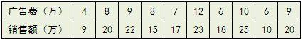
如果把广告费和销售额画在二维坐标内，就能够得到一个散点图，如果想探索广告费和销售额的关系，就可以利用一元线性回归做出一条拟合直线：

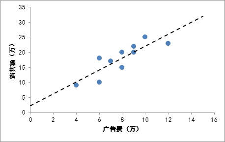
有了这条拟合线，就可以根据这条线大致的估算出投入任意广告费获得的销售额是多少。

评价回归线拟合程度的好坏

我们画出的拟合直线只是一个近似，因为肯定很多的点都没有落在直线上，那么我们的直线拟合的程度如何，换句话说，是否能准确的代表离散的点？在统计学中有一个术语叫做R^2（coefficient ofdetermination，中文叫判定系数、拟合优度，决定系数），用来判断回归方程的拟合程度。

要计算R^2首先需要了解这些：

总偏差平方和（又称总平方和，SST，Sum of Squaresfor Total）：是每个因变量的实际值（给定点的所有Y）与因变量平均值（给定点的所有Y的平均）的差的平方和，即，反映了因变量取值的总体波动情况。如下：

回归平方和（SSR，Sum of Squares forRegression）：因变量的回归值（直线上的Y值）与其均值（给定点的Y值平均）的差的平方和，即，它是由于自变量x的变化引起的y的变化，反映了y的总偏差中由于x与y之间的线性关系引起的y的变化部分，是可以由回归直线来解释的。

残差平方和（又称误差平方和，SSE，Sum of Squaresfor Error）:因变量的各实际观测值(给定点的Y值)与回归值（回归直线上的Y值）的差的平方和，它是除了x对y的线性影响之外的其他因素对y变化的作用，是不能由回归直线来解释的。

SST（总偏差）=SSR（回归线可以解释的偏差）+SSE（回归线不能解释的偏差）

所画回归直线的拟合程度的好坏，其实就是看看这条直线（及X和Y的这个线性关系）能够多大程度上反映（或者说解释）Y值的变化，定义

R^2=SSR/SST 或 R^2=1-SSE/SST

R^2的取值在0，1之间，越接近1说明拟合程度越好

代码实现

环境：MacOS mojave　　10.14.3

Python　　3.7.0

使用库：scikit-learn 0.19.2

sklearn.linear_model.LinearRegression官方库：https://scikit-learn.org/stable/modules/linear_model.html

>>> from sklearn import linear_model
>>> reg = linear_model.LinearRegression()
>>> reg.fit([[0, 0], [1, 1], [2, 2]], [0, 1, 2])#以（x,y）形式训练
...                                       
LinearRegression(copy_X=True, fit_intercept=True, n_jobs=None,
                 normalize=False)
>>> reg.coef_
array([0.5, 0.5])    #第一个是斜率，第二个是截距

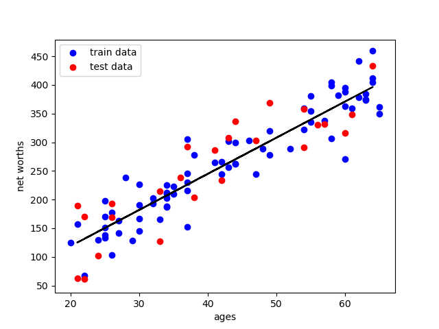
举例，以年龄与资产净值为例

图中蓝点是训练数据，用于计算得出拟合曲线；红点是测试数据，用于计算拟合曲线的拟合程度

均属于样本，仅仅是随机分离出来。

Main.py　　主程序以及画图

import numpy
import matplotlib
matplotlib.use('agg')

import matplotlib.pyplot as plt
from studentRegression import studentReg
from class_vis import prettyPicture

from ages_net_worths import ageNetWorthData

ages_train, ages_test, net_worths_train, net_worths_test = ageNetWorthData()



reg = studentReg(ages_train, net_worths_train)


plt.clf()
plt.scatter(ages_train, net_worths_train, color="b", label="train data")
plt.scatter(ages_test, net_worths_test, color="r", label="test data")
plt.plot(ages_test, reg.predict(ages_test), color="black")
plt.legend(loc=2)
plt.xlabel("ages")
plt.ylabel("net worths")

print ("katie's net worth prediction: ", reg.predict(27))  #预测结果
print ("r-squared score:",reg.score(ages_test,net_worths_test))
print ("slope:", reg.coef_)                    #获取斜率
print ("intercept:" ,reg.intercept_)              #获取截距

plt.savefig("test.png")

print ("\n ######## stats on test dataset ########\n")
print ("r-squared score: ",reg.score(ages_test,net_worths_test))  #通过使用测试集，可以察觉到过拟合等情况

print ("\n ######## stats on training dataset ########\n")
print ("r-squared score: ",reg.score(ages_train,net_worths_train))

plt.scatter(ages_train,net_worths_train)
plt.plot(ages_train,reg.predict(ages_train),color='blue',linewidth=3)
plt.xlabel('ages_train')
plt.ylabel('net_worths_train')
plt.show()

class_vis.py　　绘图与保存图像

import numpy as np
import matplotlib.pyplot as plt
import pylab as pl

def prettyPicture(clf, X_test, y_test):
    x_min = 0.0; x_max = 1.0
    y_min = 0.0; y_max = 1.0
    
    # Plot the decision boundary. For that, we will assign a color to each
    # point in the mesh [x_min, m_max]x[y_min, y_max].
    h = .01  # step size in the mesh
    xx, yy = np.meshgrid(np.arange(x_min, x_max, h), np.arange(y_min, y_max, h))
    Z = clf.predict(np.c_[xx.ravel(), yy.ravel()])

    # Put the result into a color plot
    Z = Z.reshape(xx.shape)
    plt.xlim(xx.min(), xx.max())
    plt.ylim(yy.min(), yy.max())

    plt.pcolormesh(xx, yy, Z, cmap=pl.cm.seismic)

    # Plot also the test points
    grade_sig = [X_test[ii][0] for ii in range(0, len(X_test)) if y_test[ii]==0]
    bumpy_sig = [X_test[ii][1] for ii in range(0, len(X_test)) if y_test[ii]==0]
    grade_bkg = [X_test[ii][0] for ii in range(0, len(X_test)) if y_test[ii]==1]
    bumpy_bkg = [X_test[ii][1] for ii in range(0, len(X_test)) if y_test[ii]==1]

    plt.scatter(grade_sig, bumpy_sig, color = "b", )
    plt.scatter(grade_bkg, bumpy_bkg, color = "r",)
    plt.legend()
    plt.xlabel("bumpiness")
    plt.ylabel("grade")

    plt.savefig("test.png")

ages_net_worths.py　　样本点数据

import numpy
import random

def ageNetWorthData():

    random.seed(42)
    numpy.random.seed(42)

    ages = []
    for ii in range(100):
        ages.append( random.randint(20,65) )
    net_worths = [ii * 6.25 + numpy.random.normal(scale=40.) for ii in ages]
### need massage list into a 2d numpy array to get it to work in LinearRegression
    ages       = numpy.reshape( numpy.array(ages), (len(ages), 1))
    net_worths = numpy.reshape( numpy.array(net_worths), (len(net_worths), 1))

    from sklearn.cross_validation import train_test_split
    ages_train, ages_test, net_worths_train, net_worths_test = train_test_split(ages, net_worths)

    return ages_train, ages_test, net_worths_train, net_worths_test

studentRegression.py　　线性回归

def studentReg(ages_train, net_worths_train):

    from sklearn import linear_model
    reg = linear_model.LinearRegression()
    reg.fit(ages_train, net_worths_train)
    
    
    return reg

得到结果：

同时得到：

R^2: 0.7889037259170789

slope: [[6.30945055]]

intercept: [-7.44716216]

拟合程度约为0.79，还算可以

posted @ 2019-02-27 23:47 Joeric 阅读(1632) 评论(0) 编辑收藏举报

会员力量，点亮园子希望

刷新页面返回顶部

Joeric

线性回归（regression）

公告